Machine Learning: bias and variance

Is the popular bulls-eye diagram the best graphical representation of bias and variance in a context of ML problems?

Either as an engineer or a data scientist we can all agree that no predictive model is perfect. Despite how great our model’s performance may be, the idea behind its application is to provide the best approximation of reality. Mathematically, it means that we need to minimize prediction errors. Prediction errors have two basic components: bias and variance.

Even if this is your first reading on this topic, it should be intuitive to say that an ideal model would minimize both error components, it should have low bias and low variance. On the other hand, there is a tradeoff when it comes to a model’s ability to minimize both bias and variance.

Now you are probably trying to make sense of it just as I was a couple months ago. Here is my true motivation to write this short article: my first search on this topic returned several web pages with a bulls-eye diagram aiming to translate both concepts into machine learning lingo. Looking back, I see that this representation was not as helpful as it could be. At the end of this article, you will have a more appropriate graphical representation to understand bias and variance. Feel free to save and share it!

At first glance the bulls-eye diagram is in fact helpful. Take a look at it yourself (Figure 1):

Figure 1. Graphical illustration of bias and variance by Scott Fortmann-Roe (All rights reserved).

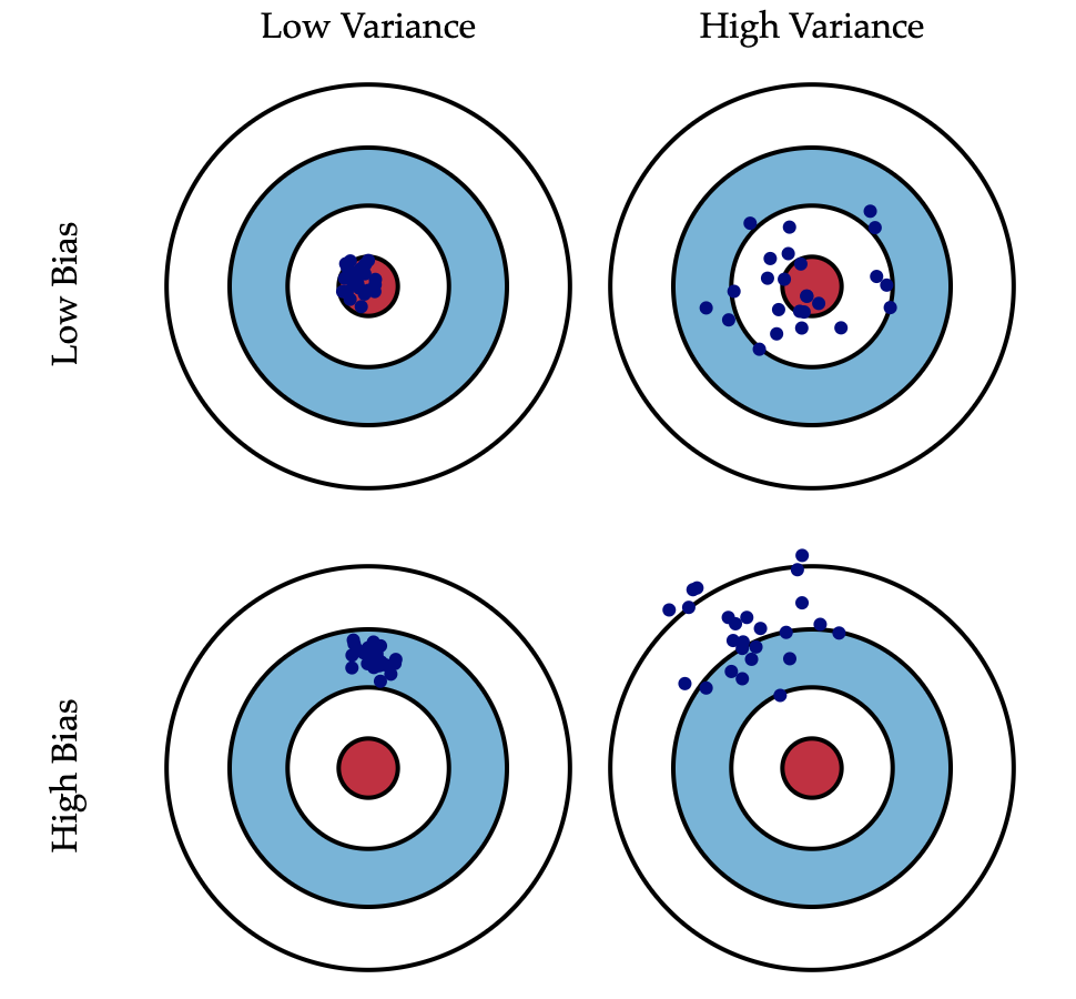
It is easy to grasp that when our predictions are far way from the bulls-eye, which represents the actual values we are trying to predict, the more substantial the prediction errors, and thus higher the bias. I quickly understood that oversimplified models are generally associated with a high bias as they fail to capture the underlying trend in the data. When our predictions are close to the bulls-eye, the smaller the prediction errors, and thus lower the bias. Complex models on the other hand are generally associated with high variance.

Let’s take a look at the statistical definition of variance on Wikipedia:

“In probability theory and statistics, variance is the expectation of the squared deviation of a random variable from its mean. In other words, it measures how far a set of numbers is spread out from their average value.”

According to this graphical illustration and the statistical definition above, variance measures the dispersion of our model predictions. In other words, if our model has low variance, we have predictions condensed into a smaller area of our target. If our model has high variance, it means our predictions are spread out. The bulls-eye diagram even allows you to infer the behavior of an ideal ML model: low bias and low variance as we first discussed. It is definitely a great starting point! Yet, here are some questions for you:

• How do we intuitively relate the bulls-eye diagram with the training and test sets?
• Is the classic definition of variance indeed helpful in a context of Machine Learning problems?

As a beginner, I had no answers to these questions. Later on, I came across an explanation that made me finally understand the bias and variance tradeoff. Here is a recommendation: StatQuest on Youtube! On his channel, Josh Starmer uses a different graphical approach and clearly explain bias and variance in no more than 6 minutes. You can check out this legend yourself or just bear with me while I try to be just as clear as he was. The following explanation, image and analysis are an adaptation of the StatQuest video.

Keep your eyes on Figure 2 as we go! As Josh would say: “Don’t sweat it!”.
We are only trying to fit a model in order to predict a mouse’s height given its weight. Our dataset is represented by the gray data points. We split our dataset into training and test sets. Blue data points represent our training set and the green data points represent our test set. Our goal is to fit the best model, a model that results in low bias and low variance. The prediction errors are represented by the red line, which measures the difference between the predictions and the actual values. They are drawn only for the test set analysis as we are usually interested in our model’s performance on unseen data (test set).

Figure 2. Bias and variance representation adapted from StatQuest.

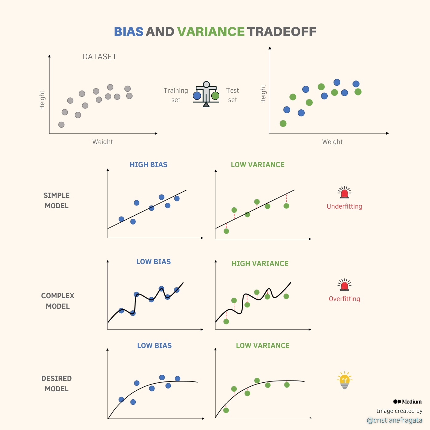
Let’s start with a linear regression model by fitting a straight line to the training set. You can see that the straight line does not fit perfectly the data, so we could compute prediction errors (also called residuals) on the training set, thus we can prove that our model has a relatively large amount of bias. Let’s define bias as the model’s inability to capture the true relationship between variables. In order to reduce bias, we can try to fit a more complex model to the training set: a squiggly line that fits the training set almost perfectly. Great, now the sum of residuals on our training set is very close to zero! What about our test set? Well, we can see that the straight line gives us consistently good predictions on both training and test sets, but they are clearly not great predictions. The squiggly line, on the other hand, give us great predictions on the training set, but they are considerably worse on the test set.

Now, it is time to give a more appropriate definition to variance in machine learning lingo. Let’s define variance as the model’s ability to produce consistently good predictions across different datasets. Considering this particular dataset, we can see that the simple model does a much better job generalizing to unseen data (test set) than the complex model.

We must keep in mind that an overly simplified model may lead to underfitting, as we might fail to capture the true relationship between variables. As we can see, there is a point where no matter how much a mouse’s weight increases, there is no effect on the mouse’s height. A straight line will never be able to reproduce this relationship. On the other hand, a too complex model may lead to overfitting since the model fits the training set so well it is unable to make consistently good predictions on unseen data. The desired model is an optimal point, a balance between a simple model and a complex model. By inserting an amount of bias into our complex model, the desired model has a significant drop in variance. Hopefully, now you have a solid intuition about bias and variance in a context of ML problems! BAM!

Thanks for reading! See you soon!